Some history and background
The brightest compotent in zeta Ursae Majoris (Mizar A) was the first spectrosocpic binary star that was discovered. It was found by Edward Pickering in 1887. The second discovery was Beta Aurigae, found by Antonia Maury in 1889. Maury was one of many women in "Pickerings computer team", that were analyzing spectra. Annie Jump Cannon and collaborators (Henrietta Leavitt, Williamina Fleming, Antonia Maury, and others) defined the current spectral classes O,B,A,F,G,K,M, based on thousands of star spectra.With these discoveries in mind, these relatively bright spectocopic binaries are also the first natural targets for hobby spectroscopists. The two components have comparable magnitudes, so that the recorded spectrum is a superpositon of two equally bright spectra that are blue-shifted and red-shifted with an amount depending on the radial velocites at the time of observation. These are called double-line spectra. If one component is very dim relative to the other, then the spectrum appears to be single lined, and the Doppler shift can only be detected after careful wavelength calibration, and the revolution can be confirmed only over time. Double-line spectra are therefore better to start with than single line spectra, as one can measure the relative Doppler shifts "instantaneously", once the dispersion (wavelength increment per pixel) is known.
Beta Aurigae with QCSPEC, April 2014 (lagging Antonia Maury by 125 years!)
The following images show the double Hydrogen alpha line in beta Auriga, due to the different line of sight Doppler shifts. This was accomplished after 4-5 nights of patient trial and error (sometimes frustration) with spectrograph adjustment, tracking, and focusing. The bottom line is that one has to be very careful with calibration of all the settings: focus, grating position, finder scope, and guider telescope -- all in a sensible order.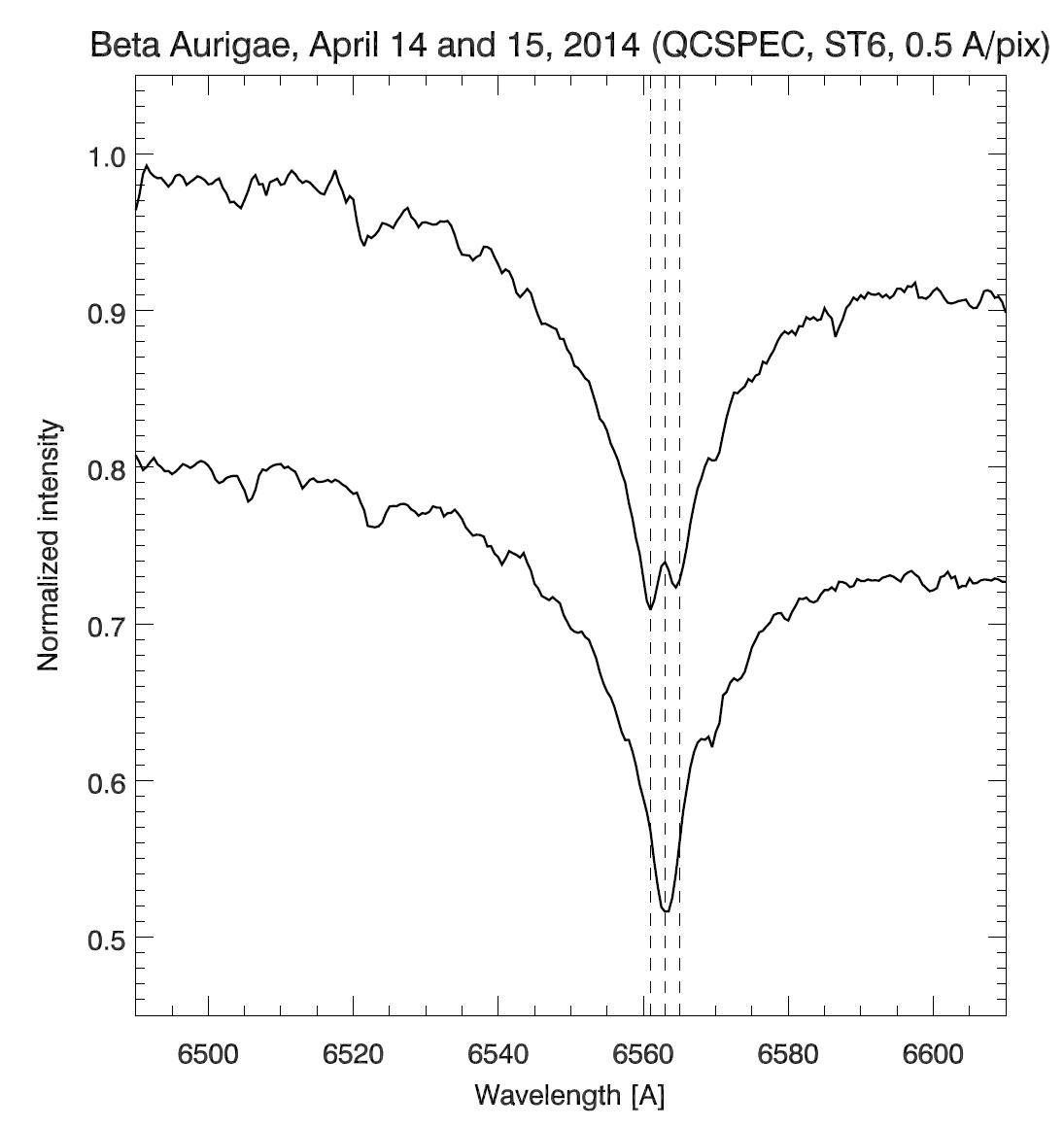
I can honestly say that Im really proud of this plot, after all the struggle. The upper spectrum shows a clear line split in hydrogen alpha, on April 14, when the stars moved roughtly along the line of sight. The lower spectrum from April 15, shows overlapping lines (no apparent Doppler shift) when the stars moved roughly tangentially to the line of sight. This timing was pure luck. Since the period is about 4 days, a one day delay between the measurments corresponds to a transition between maximum and minimum line of sight velocity, and hence the changes seen.
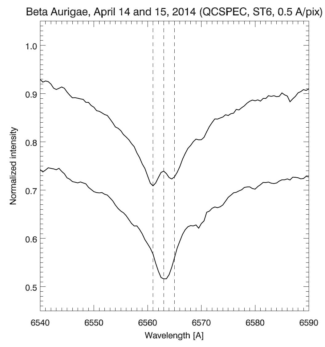
This zoom-up shows that the red- and blue-shift is about 2 Angstroms, which corresponds to the expected orbital velocities of the order of 100 km/s. This implies that the (upper) spectrum was (luckily) recorded near the maximum line of sight velocity! A closer look reveals that the Doppler shifts are possibly not identical for the two components (and this may be expected), but the measurement uncertainty (with the noise level) tells me that such a statement is too bold, and we can say that the Doppler shift for both is about 2 Angstroms. A further analysis is given below. The upper spectrum was averaged over six exposures, and the lower spectrum was averaged over 23 exposures. Each exposure was 90 seconds, giving 9 and 34 minutes total exposure times. A single exposure is shown below. The spectra shown above are smoothed over three pixels along the wavelength axis to suppress the remaining thermal and photon noise.
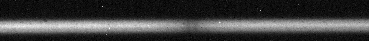
A single raw image from the ST6, of 90 seconds exposure time, showing the split hydrogen alpha line. Some noise and hot pixels is seen, and some bright streaks due to slight drift in and out of the slit (the latter does not degrade the spectra much). Each spectral image is averaged in the vertical direction, but only over the bright strip where we have a significant signal, and this generates the spectra above.
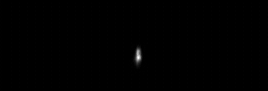
A 5 second exposure of the slit in the zero order spectrum, slows that the slit appears to be only a couple of pixels wide. More details on the Doppler shift measurements and their meaning can be found further below. But first, we will look more into the equipment that was used.
Equipment and challenges
My experiene is that it is very challenging to obtain good quality spectra that clearly reveal the line-split (challenging, relative to the rest of the bright star work shown on this web page). Success is then even more rewarding! I found that: 1) The slit has to be very narrow for sufficient spectral resolution. 2) Accurate guiding is therefore necessary, to center the diffraction disk on the narrow slit. If not, then we loose photons. 3) The stars are not very bright, so a light sentitive CCD is required (rather than an ordinary digital camera, which I also tried). So, this can really add up and become expensive. However, Im keen on keeping things cheap if possible, and use home made stuff, or old stuff that I already have.I used (a now "old", I suppose) ST6 camera from the early 90's, and a guiding telescope with an inexpensive MEADE LPI imager. The CCD is borrowed from a local astronomy club, with the acronym GoTAF. The guiding refractor has a 60 mm opening and with a 2x barlow lens, the effective focal length is 1800 mm. This provides the needed sensitivity (or "plate scale") for accurate guiding. The guiding telescope (a Vesper Optics, from the early 60's) was kindly given to me by my neighbor, Hans Brubak, as he was thinking about getting a modern telescope. The stellar live image from the guider camera was traked manually on the computer screen, by using the telesope controller (via arrow keys on the computer keybord). The stepper motor controller was home made, constructed, and programmed by Ragnar Kalleberg in the early 90's, and I still use it with my first decent computer from 1990, a 286 Unisys home PC (if ain't broke, don't fix it: back then, computer technology was made to last and to serve people - haha).
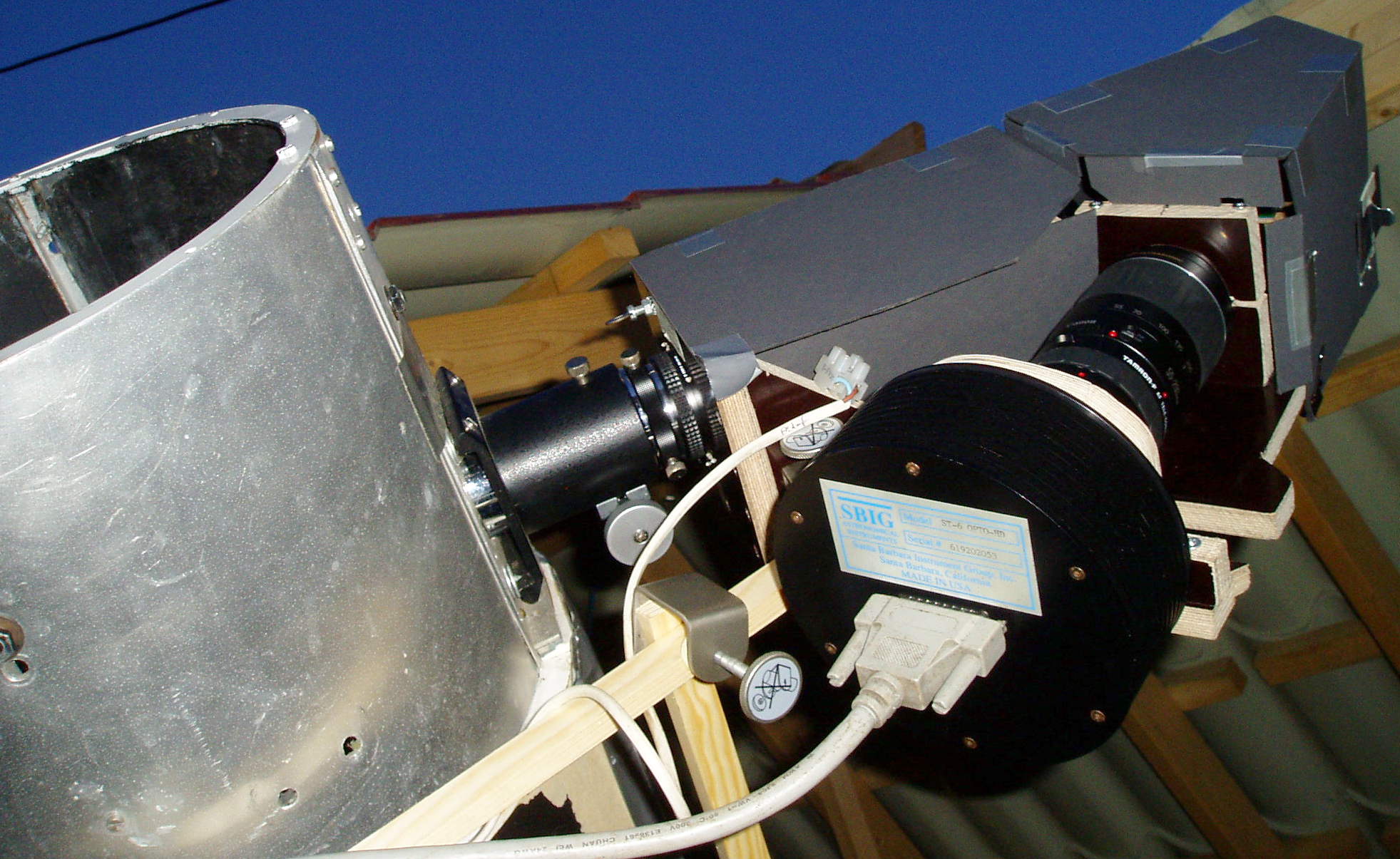
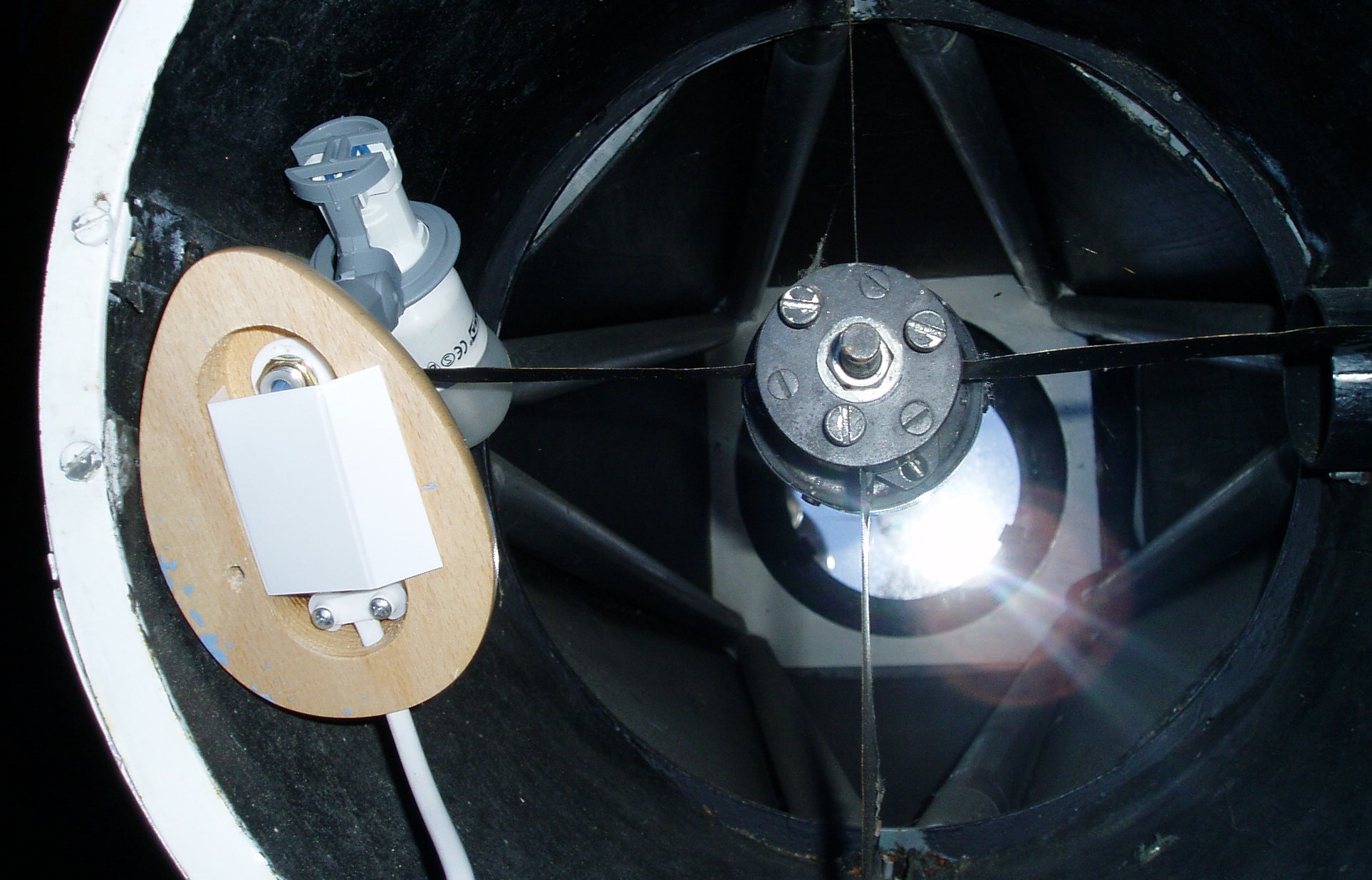
Left: My home made "QCSPEC" spectrograph and the antique ST6 CCD camera on the home made 10 inch Newtonian telespoce (first owned by Jacob Lingaas at Lillehammer). Right: A fluorescent light bulb was dropped inside the telescope to image the slit in the zero order spectrum, to make sure that the slit was in focus on the CCD chip.
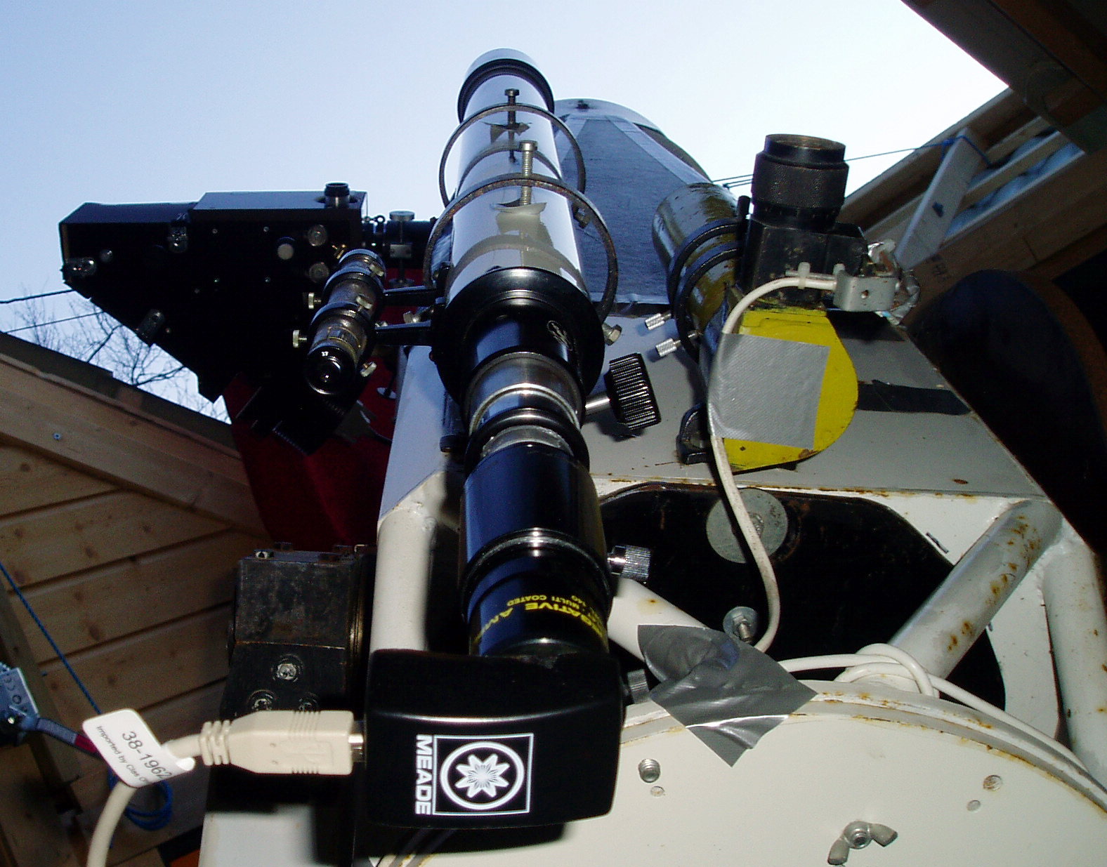
A "collectible" Vesper Optics 60x900 refractor from the early sixties, with 2xBarlow lens in front if an LPI guider. The smaller 7x50 type finder scope (yellow) has a red illuminated cross hair system.
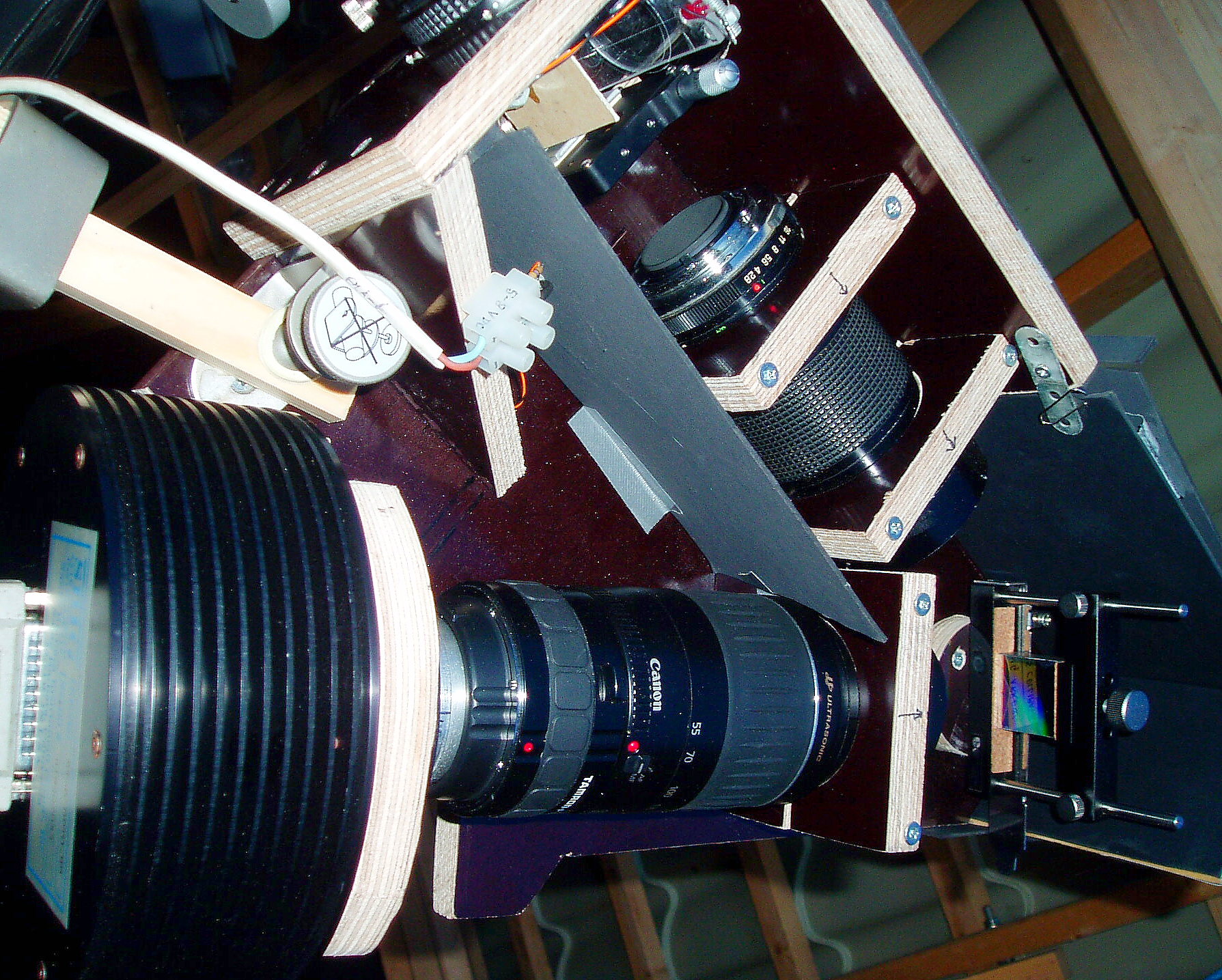
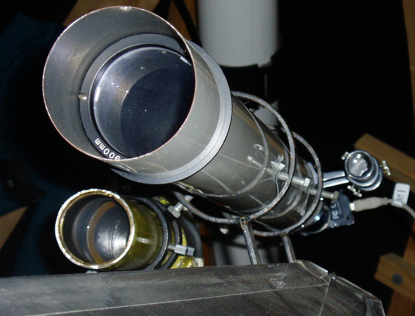
Inside the spectrograph. From the upper left and clockwise: 20 micron slit, collimator (90mm f/2.8 lens), 30x30mm 1200 lines/mm grating, camera lens (200 mm with 2x teleconverter), ST6 CCD camera (cooled to -30 or -40 degrees centigrade). This setup gives 0.5 Angstrom per pixel, and sufficient light sensitivity for less bright stars. The black-and-white 16 bit ST6 has relatively large pixels (23x27 microns), and it is therefore quite light sensitive, and stand up to modern CCD's in this respect.
Comparison to calcuated velocity curves for beta Aurigae
For binary stars systems, one can do exact calculations and predictions, due to their simple and deterministic character. The resulting equations can be found elsewhere (e.g. in the excellent notes by Kelsey Clubb of San Francisco State University, where she shows all the calculation steps. This is available on the web). The shape of the calculated velocity curves depend of the orbital elements of the system (eccentricity of the orbits, inclination and orientation of the orbits relative to the "sky plane" (tangntial to the celestial sphere), and the semi-major axes of the two ellipses about the center of mass. The ratio of the latter two quantities is equal to the mass ratio of the stars. By tuning the calulated curves so thay fit the data, one can deduce some of the orbital elements, such as the eccentricity. The individual masses can only be found if the inclination of the orbits are known as well, by other means.A comparison between the current measurements, and the observations and calulations of Behr et al. (2011)(axXiv:1104.1447v1), are shown below. The rectangles represent the uncertainty in the current data, and we estimate the uncertainty in the Doppler shift to be about 0.5 Angstom, which translates into an uncertainty of about 20 km/s. From the shift of the spectral lines in the plots (roughly 2 Angstroms), we estimate the radial velocities to be +90 km/s (red shifted) and -90 km/s (blue shifted). This shift is measured relative to the central wavelength of the single line (bottom curve in the spectra above), so this implies measured velocities relative to the radial velocity of the center of mass of the system. The phase increment from 0 to 1 corresponds to the orbital period of 3.98 days, and the measurements were done about 24 hours apart (1/4 or a full phase, as shown by the separation beteen the rectangles).
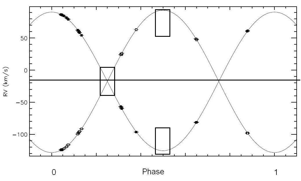
The calulations (lines) and datapoints from Behr et al. (2011) (axXiv:1104.1447v1) for beta Aurigae are shown, together with the current measurements. The rectangles represent the uncertainty in the current measurements, and the center of the rectangles represent the estimated Doppler velocities from the spectra above. The data from Behr et al. (2011) is very accurate in comparison. The center of mass of this system approach the Sun with a velocity of -17 km/s (blue shift), and this is seen where the velocity curves cross each other (when the two lines overlap the stars move tangentially to the line of sight, and there is no radial orbital motion). The velocity data of Behr et al. is calibrated with the Sun as the refece point, and we may calibrate our data similarly.
Mizar A
The A-component of Mizar is also a possible hobby project, although this star is slightly less luminous (mag 2.3):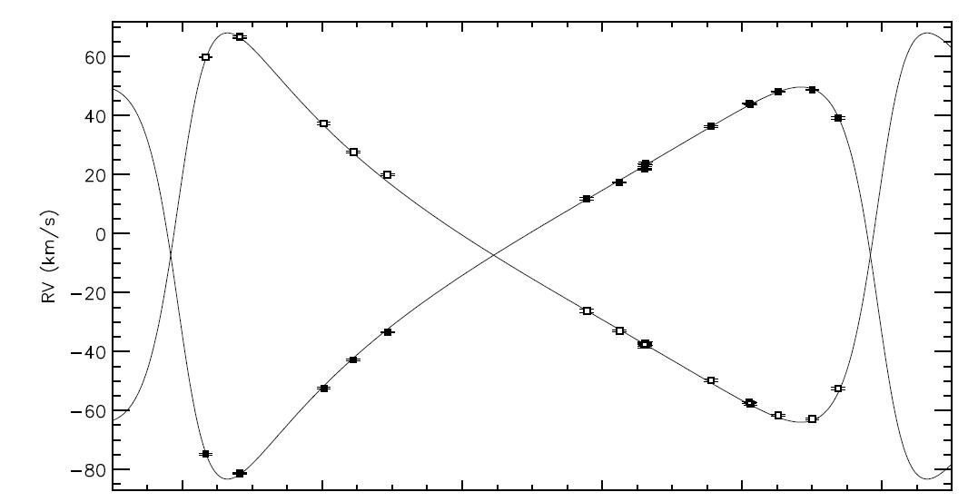
The calulations (lines) and datapoints for Mizar is also from Behr et al. (2011) (axXiv:1104.1447v1). The shape of the radial velocity curve is very sentitive to the orbital elements (eccentricity (e), inclination (i) with the sky plane, and the angle (w) between the ascending node of the sky plane and periastron). The orbits are now strongy elliptical with an eccentricity of at bout 0.54, giving sawtooh shaped velocity curves, whereas for beta Aurigae, the eccentricity is near zero, giving almost sinusoidal curves.
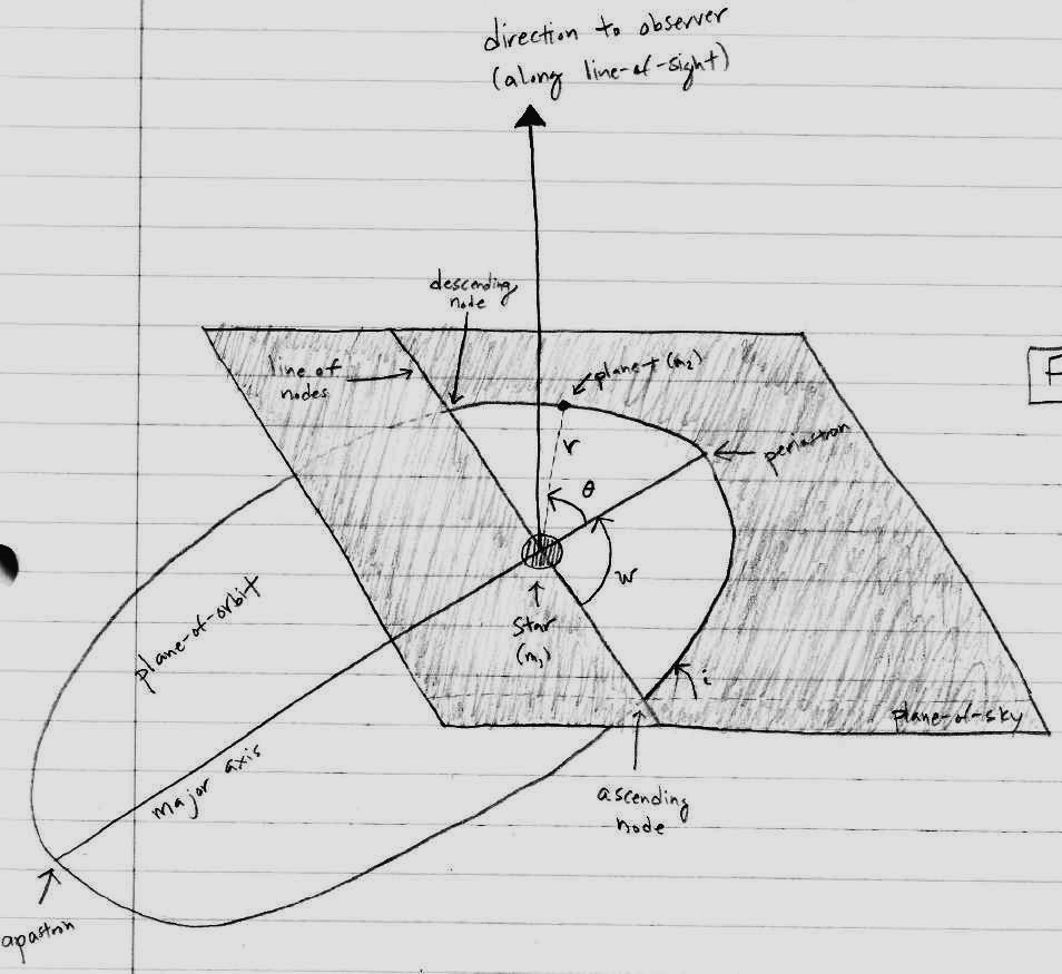
The orbital elements (borrowed from Kelsey Clubb and her note "The Radial Velocity Equation": this is available on the internet. Thanks, Kelsey!).